Which neural network works best for quadratic hedging?

The Problem

This paper does not propose a new hedging algorithm. It systematically evaluates three deep learning architectures for quadratic hedging: Multi-net, Single-net, and RNN. The main question is which architecture is more reliable for high-dimensional, long-horizon dynamic hedging.

The second contribution is a model-free moving block bootstrap method for generating training data from historical paths, together with an empirical study of how block size affects the result.

Objective

Let there be $d$ underlying assets with price vector $\boldsymbol S_t\in\mathbb R^d$. The hedging position at time $t$ is $\boldsymbol q_t\in\mathbb R^d$, and the initial capital is $v$. Terminal hedging wealth is:

$$V_t = v + \sum_{i=0}^{t-1} \boldsymbol q_i^\top (\boldsymbol S_{i+1}-\boldsymbol S_i).$$

The payoff used in the experiments is a European basket call:

$$F_T = \left( \sum_{j=1}^{d} S_{j,T} - dK \right)^+.$$

Quadratic hedging minimizes the mean squared terminal hedging error under the real-world probability measure:

$$\min_{v,\boldsymbol q_0,\ldots,\boldsymbol q_{T-1}} \mathbb E \left[ (V_T-F_T)^2 \right].$$

If a neural network outputs each hedge, then:

$$\boldsymbol q_t = f_\theta(X_t),$$

where $X_t$ is the observable state at time $t$. Training uses sample average approximation:

$$\widehat L(\theta) = \frac{1}{M} \sum_{m=1}^{M} \left( v_\theta + \sum_{t=0}^{T-1} f_\theta(X_t^{(m)})^\top \Delta \boldsymbol S_{t+1}^{(m)} - F_T^{(m)} \right)^2.$$

All architectures solve this same objective. The difference is how they represent $\boldsymbol q_t$. To isolate architecture effects, the main problem does not include transaction costs or position constraints.

The three architectures

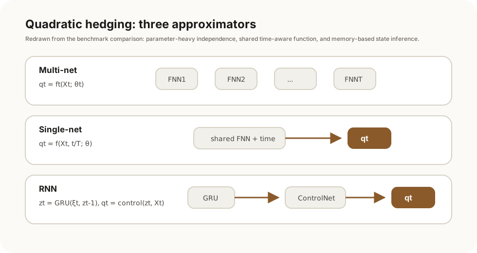
Multi-net uses a separate network for each time:

$$\boldsymbol q_t = f_t(X_t;\theta_t).$$

It has the most flexibility, but its parameter count grows linearly with the horizon $T$. The paper finds that this causes overfitting and training instability in high-dimensional, long-horizon settings.

Single-net uses one shared network and gives normalized time as an input:

$$\boldsymbol q_t = f(X_t,t/T;\theta).$$

Its parameter count does not grow with $T$, making it the smallest and fastest of the three architectures.

RNN reads the history of returns. With log return $\boldsymbol\xi_t$ and hidden state $\boldsymbol z_t$:

$$\boldsymbol z_t = \mathrm{GRU}(\boldsymbol\xi_t,\boldsymbol z_{t-1};\theta^R), \qquad \boldsymbol q_t = f^C(\boldsymbol z_t,\tilde X_t;\theta^C).$$

The paper uses GRU rather than LSTM, since LSTM did not bring clear improvement and was slower. A key design choice is to feed log returns $\boldsymbol\xi_t$ into the RNN cell rather than prices $\boldsymbol S_t$, then use a ControlNet to map the hidden state to the hedge.

Market Models

The paper uses two data-generating models.

Black-Scholes. Log returns are i.i.d. multivariate normal. In this setting, the price process is relatively simple and $\boldsymbol S_t$ can serve as a Markov state.

DCC-GARCH. Volatility and correlation evolve over time, producing volatility clustering, fat tails, and changing correlations. In this setting, prices alone do not fully describe the state, and the hidden covariance state is not directly observable in real trading.

This is why RNN is relevant: when the market state depends on historical returns, an RNN may extract part of the hidden state from $\boldsymbol\xi_{1:t}$.

Experimental Design

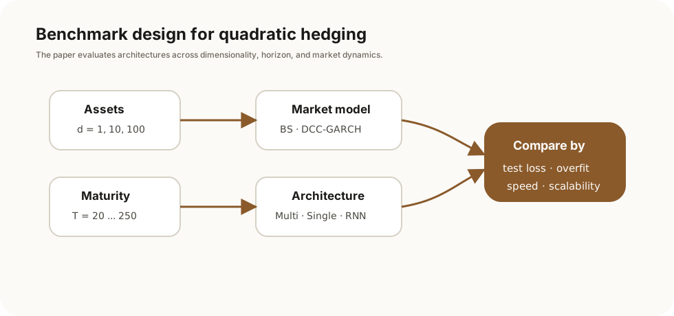
The benchmark varies asset dimension $d\in\{1,10,100\}$, maturity $T\in\{20,60,120,250\}$, and market model. Each setting compares Multi-net, Single-net, and RNN.

Training uses PyTorch, Adam, minibatches, validation selection, and gradient clipping. The paper also applies several stabilization steps: using $\log(S_t)$ instead of $S_t$, standardizing features, using $v/d$ as a training parameter, and dividing the loss by $d^2$ so that the same training setup can work across dimensions.

Risk-neutral price $p$ and initial delta $\Delta_0$ are used as references. The paper emphasizes that they are not the true answers to this real-world-measure quadratic hedging problem, especially under incomplete DCC-GARCH dynamics.

Main Findings

In low dimension, the architectures are similar. For $d=1$, the three methods converge to similar training and test loss. The differences appear mainly in high-dimensional and long-horizon settings.

Multi-net overfits. Its parameter count grows with $T$. In large settings such as $d=100,T=250$, it reaches millions of parameters, and validation loss can be much higher than training loss. Training is also unstable under DCC-GARCH.

RNN usually has the lowest test loss. The advantage is especially clear under DCC-GARCH. The paper explains this by the RNN’s ability to extract information about unobservable dynamic covariance states from historical returns.

Single-net is a strong baseline. It is small, fast, and resistant to overfitting, and in many cases its test loss is only slightly worse than RNN. The paper therefore compares accuracy and stability rather than claiming that RNN dominates every practical consideration.

Learned $v$ and $\boldsymbol q_0$ can differ from risk-neutral price and delta. In high dimensions, the learned initial capital and hedge can deviate substantially from $p$ and $\Delta_0$. The paper’s point is not that classical formulas are wrong, but that they solve a different objective.

Moving Block Bootstrap

The paper also studies model-free training data generation. It samples moving blocks of length $b$ from a historical path and concatenates them to create training paths.

The block size controls the trade-off. When $b=1$, the method becomes IID bootstrap. Larger $b$ preserves more temporal dependence, but it reduces sample diversity. In the paper’s DCC-GARCH study, small block sizes, including $b=1$, give the best RMSE for $v/d$ and $\boldsymbol q_0$. RNN also has lower $\boldsymbol q_0$ estimation error than Single-net under small blocks.

My Discussion

My own interpretation belongs here. The paper’s value is not that it proposes a new hedger, but that it gives a careful architecture benchmark. It shows that memory helps when market state is partially observable and time-varying, while Single-net remains an important simple and stable baseline. The omission of transaction costs and position constraints is intentional for isolating architecture effects, but it also means the setup is not a complete trading system.