Deep learning for enhanced index tracking
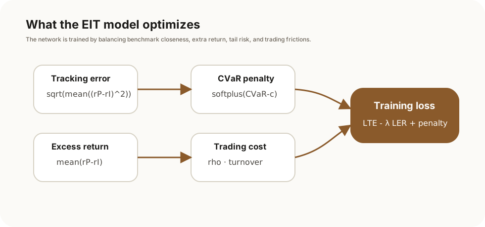
This paper formulates enhanced index tracking as a dynamic rebalancing problem: select large index constituents, then let a structured neural network allocate weights under tracking-error, excess-return, CVaR, and transaction-cost considerations.
The Problem
Index-related funds include two related but different tasks. Index tracking minimizes tracking error relative to a benchmark. Enhanced index tracking tries to obtain excess return while controlling tracking error.
The article studies enhanced index tracking and treats ordinary index tracking as a special case. The portfolio trades index constituents and cash. The workflow has two steps: stock selection and weight allocation. For stock selection, the method uses a transparent criterion: select large constituents of the S&P 500 by free-float market capitalization. The main research problem is the second step, how to dynamically allocate weights among selected stocks and cash.
Conventional weight allocation is usually formulated as a single-period optimization problem. It uses recent one- or two-year returns and periodically re-optimizes. The drawback is that such a policy may not catch up with regime switches. The proposed alternative is a neural-network-generated dynamic rebalancing policy.
Why Not A Large Black Box
The paper identifies three concerns for neural-network policies in this problem.
First, real market data are limited compared with other deep learning domains, so overly sophisticated models can overfit. Second, scalability matters: directly feeding stock features into a standard FNN creates a large network when the number of stocks grows. Third, an investment policy needs some interpretability.
The contribution is therefore not a larger network. It is a small structured architecture with four blocks: main, score, gate, and memory. These blocks use different features, share parameters where possible, and incorporate transaction cost, no-short-selling, no-leverage, and CVaR control.
Control Variables And State Dynamics
Suppose stocks have been selected. The pre-trade weight vector at time is:
where is the cash weight. The post-trade weight vector is:
The current portfolio value is normalized to 1. With proportional transaction cost ratio , post-trade weights satisfy:
The control variable is the stock-weight vector , subject to no short selling and no leverage:
The next-period portfolio return is:
Transaction cost is therefore not an after-the-fact deduction. It directly enters realized return and the state transition. The state is the initial weight at and then includes portfolio return and current weights.
The EIT Objective
The paper assumes that portfolio and index returns are stationary. The first objective is the root mean squared tracking error of daily returns:
The second objective is mean daily excess return:
The EIT objective is:
When , the problem becomes ordinary index tracking. In the experiments, IT uses and EIT uses . This value is chosen because daily tracking error is around the scale while daily excess return is around the scale; without a relatively large , the excess-return term would be underweighted.
CVaR Control
The paper then controls downside risk. Given the return distribution , VaR and CVaR are defined as:
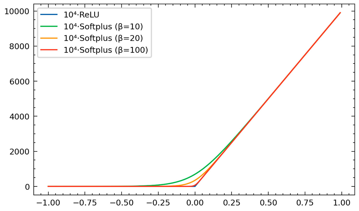
Adding directly is difficult in deep learning, so the paper converts it to a penalty:
Instead of a ReLU penalty, the paper uses the Softplus function:
The EIT-CVaR objective is:
For the S&P 500 experiments, the paper sets , , , , and . The value corresponds to the pre-test historical 95%-CVaR level of S&P 500 daily returns.
Features
The network uses four classes of features.
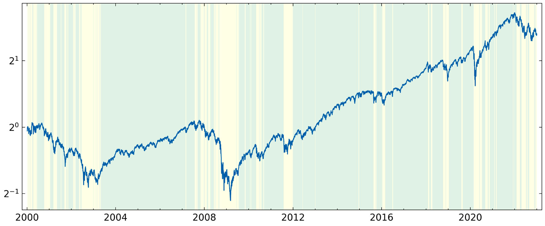
The first feature is the index regime probability. The paper fits a two-state HMM for the index and uses the forward algorithm to filter:
The second feature is stock regime probability:
These probabilities are smoothed by recent averages, giving and .
The third feature class contains short-term features: recent mean, volatility, and beta for each stock, plus recent mean and volatility for the index. The fourth feature is the current stock-weight vector , used for transaction-cost control.
Four Network Blocks
The key architecture consists of four blocks: main, score, gate, and memory.
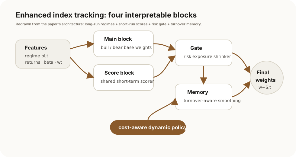
The main block learns a bull allocation and a bear allocation. It obtains and through softmax, then mixes them using the bull-regime weight :
The score block scores each stock using short-term features. Since its parameters are shared across stocks, network size does not grow excessively with the number of stocks. It produces , then mixes it with the long-term allocation:
The gate block uses stock regime probabilities to generate and scale candidate weights stock by stock:
The memory block is used only when . It reads the distance between proposed and current weights and outputs , canceling part of the proposed weight change:
The networks are small: main, gate, and memory are ; the score block is . Hidden layers use GELU. The main, gate, and memory outputs use Sigmoid; the score output is real-valued.
Experimental Setup
The S&P 500 experiment uses daily adjusted closing prices from January 3, 2000. The stock universe is the top-20 S&P 500 constituents by market cap before the test period, with stocks listed after January 3, 2000 filtered out. Cash return is assumed to be zero.
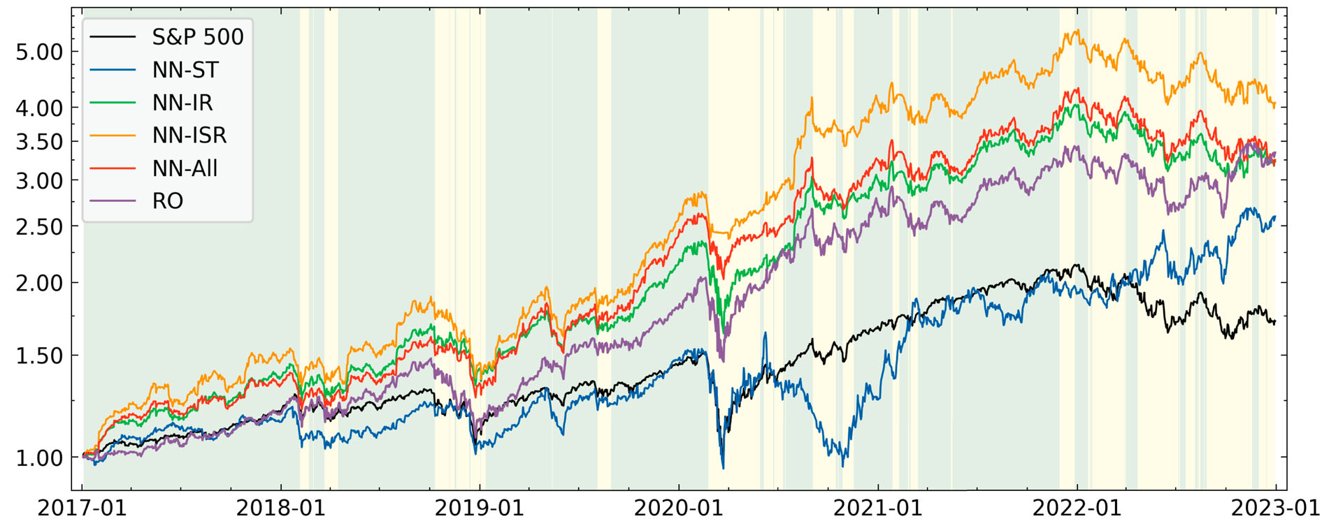
Training and testing follow a rolling scheme: train on 2000-2016 and test on 2017; train on 2000-2017 and test on 2018; continue through 2022. Each year, HMMs are refitted and neural-network policies are retrained.
There are three tasks: IT, EIT, and EIT-CVaR. There are two stock counts: top 5 and top 20. There are two transaction-cost settings: and , or 50 basis points. The rebalancing period is trading days because it gives similar excess-return and CVaR performance to daily rebalancing with much lower transaction costs.
The paper compares five policies: four neural-network policies and one re-optimization benchmark.
| Policy | Features | Blocks |
|---|---|---|
| NN-ST | Short-term features, current weights | score, memory |
| NN-IR | Index regime, current weights | main, memory |
| NN-ISR | Index regime, stock regime, current weights | main, gate, memory |
| NN-All | Index regime, short-term features, stock regime, current weights | main, score, gate, memory |
| RO | Rolling recent-data optimization | conventional benchmark |
Performance metrics include TE, MER, IR, CR, Sharpe ratio, loss, 95%-CVaR, MDD, and ATC. The return measures are calculated after transaction costs.
IT: Limited Neural-Network Advantage
For ordinary index tracking, all policies track the index trend over the long run. With five stocks, NN-ST has the smallest TE; with twenty stocks, RO is the best.
The paper’s explanation is that IT is a regression-type problem. The RO baseline already constructs a strong tracking portfolio, so there is limited room for improvement by a more sophisticated model.
EIT: Regime Features Become Important
When the excess-return objective is added, the conclusion changes. NN-ISR, which uses both index and stock regime probabilities, outperforms the others in MER, Sharpe ratio, and CR in all four S&P 500 cases. This indicates that regime information is more important for EIT.
NN-IR and NN-All also perform well in return measures, with NN-IR achieving the best IR in three out of four cases. By contrast, NN-ST, which only uses short-term features, performs poorly in returns and is the riskiest.
The weakness of EIT is also clear: it does not directly control risk. All policies have higher 95%-CVaR than the index, and MDD can be large. The paper therefore moves to EIT-CVaR.
EIT-CVaR: Lower Risk At A Return Cost
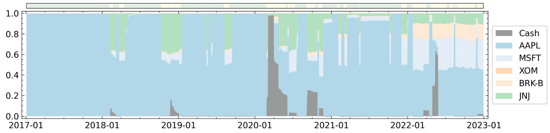
After adding the CVaR constraint, all 95%-CVaR values are controlled below 3%. MDD also decreases relative to EIT, although it is not directly constrained.
The cost is lower return: smaller risk is paid for with smaller returns. RO becomes overly conservative in EIT-CVaR, holding too much cash for too long and producing poor return performance. NN-IR and NN-ST are also conservative. NN-ISR and NN-All still perform well in MER, IR, Sharpe ratio, and CR.
Reading The Weights
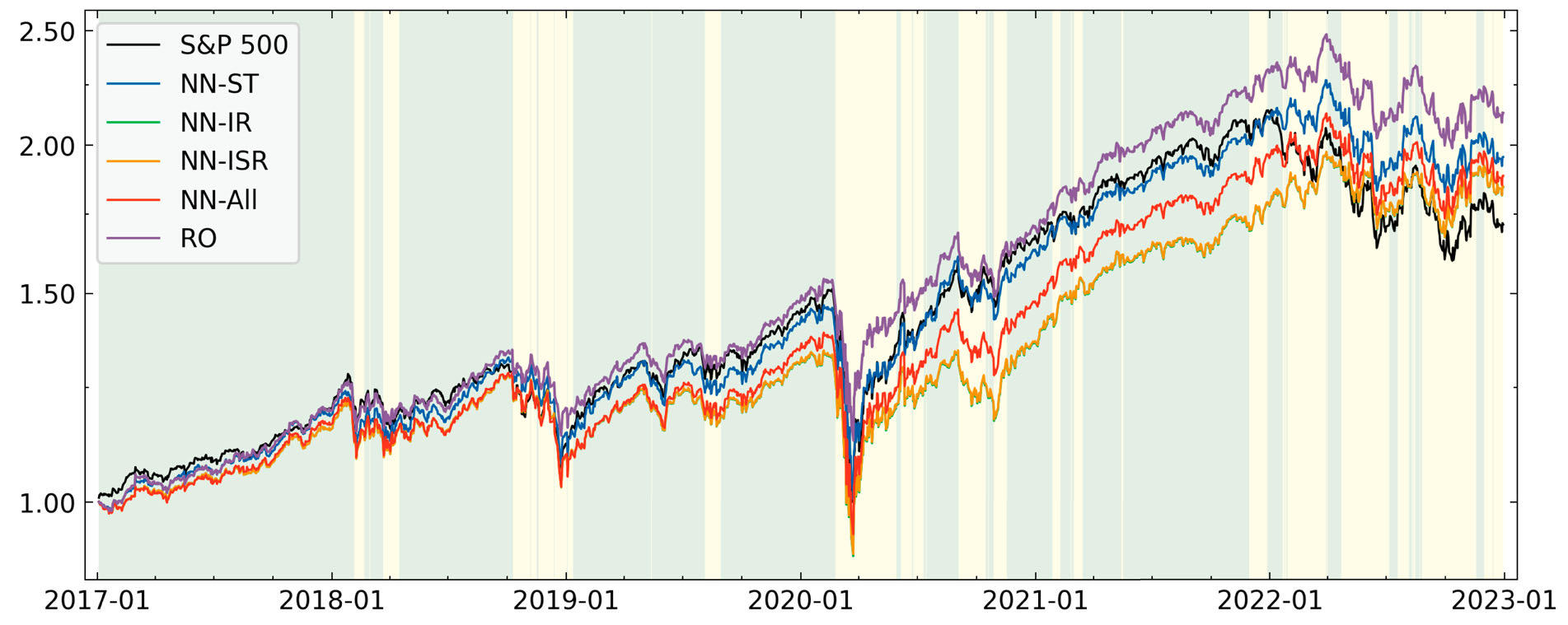
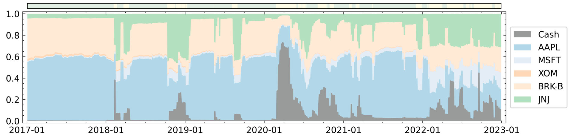
The rebalanced-weight figures are central to the paper’s interpretation.
For IT, policies tend to invest in stocks and cash more evenly and update weights slowly. The good performance of NN-ST is credited to the score block.
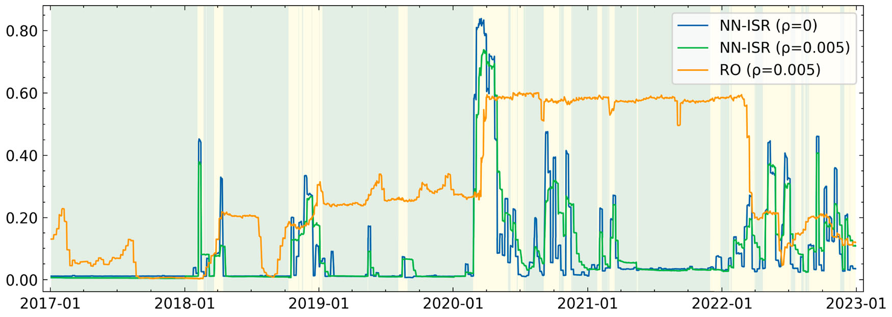
For EIT and EIT-CVaR, policies tend to concentrate on selected stocks. The CVaR penalty leads to more diversification, but AAPL still receives a large weight under NN-ISR and NN-All. NN-ISR and NN-All show flexibility: they hold more high-return stocks in bull markets and more cash in bear markets. The rise in cash weight during the 2020 market meltdown is the flight-to-safety behavior emphasized by the paper.
RO cannot fly to safety well in EIT. In EIT-CVaR, it can increase cash, but then remains heavily invested in cash long after the recovery. NN-IR uses only index regime and can also switch weights, but its flight to safety is less obvious than NN-ISR’s. This shows why the gate block and stock regimes matter.
What The Blocks Learn
The paper also plots input-output curves of the learned blocks.
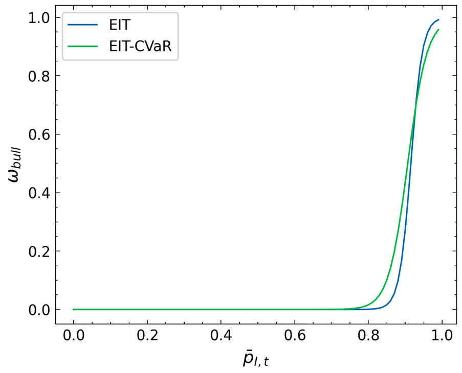
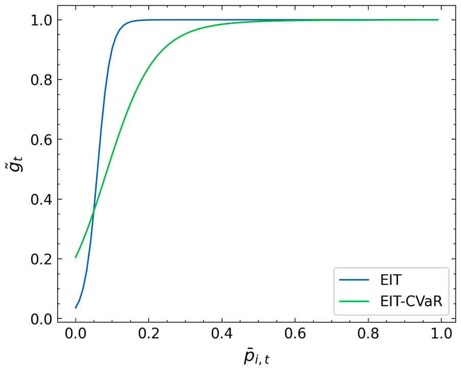
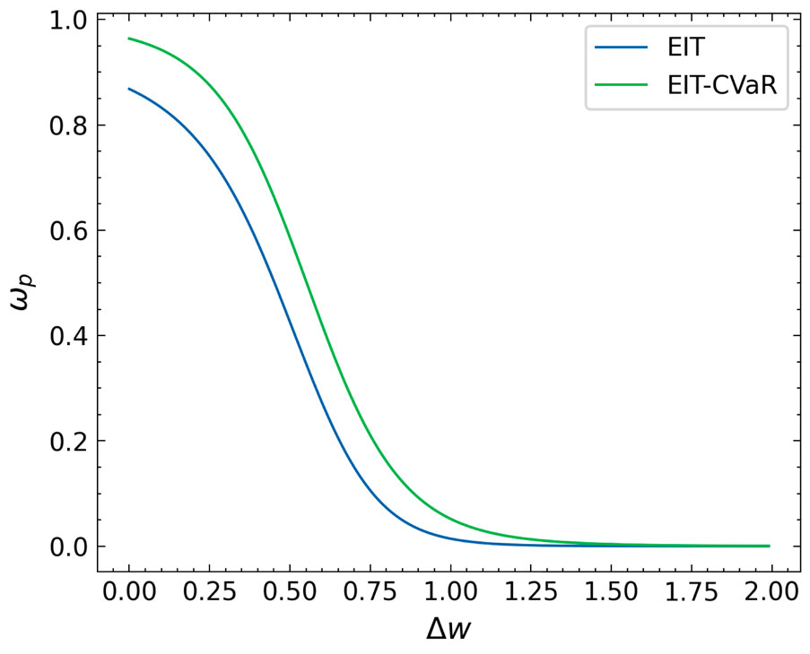
These curves support the paper’s feature-importance conclusion: short-term features are most useful for IT, while both index and stock regime probabilities are important for EIT and EIT-CVaR.
Transaction Costs
In IT, transaction costs are low because weights change slowly. In EIT and EIT-CVaR, neural-network policies change weights more dramatically and frequently, so transaction costs matter.
The conclusion is not that transaction costs destroy the neural-network policies. Policies with appropriate features still outperform RO, and the best-return policy, NN-ISR, is not the most costly one. This supports the role of the memory block.
Cross-Market Extension
The paper also tests EIT-CVaR with transaction costs on S&P 100, FTSE 100, and Nikkei 225, using . Training starts in 2003, testing covers 2019-2023, and CVaR constraints are set to 3%, 2.7%, and 3.3%.
Except for the five-stock cases of FTSE 100 and Nikkei 225, NN-ISR has lower test loss and higher CR and Sharpe ratio than RO in 7 out of 9 cases. It also has higher MER and IR in 8 out of 9 cases. The paper therefore treats the improvement over RO as reasonably robust to changes in index and stock count.
The Nikkei 225 case is a warning. Both NN-ISR and RO fail to generate excess CR over the index. The paper gives two reasons: selected large-cap Nikkei stocks perform poorly, and the CVaR constraint makes the strategy more conservative. Further work is needed on stock selection when large-cap stocks do not perform well.
Conclusion
The paper’s conclusion can be summarized in five points.
First, it proposes a data-driven deep learning method for dynamic EIT rebalancing. Second, it introduces index and stock regimes as features and finds them key to investment performance. Third, it designs the architecture to be parsimonious, scalable, easy to train, and more interpretable. Fourth, empirical results verify the advantage over conventional RO. Fifth, the framework is flexible enough to incorporate additional features and constraints.
Notes
From a reader’s point of view, the paper is not about deep learning magically selecting stocks. Stock selection is still market-cap based. The innovation is in weight allocation: regime information, CVaR, transaction cost, and memory are built into a dynamic control framework.
The main reusable ideas are therefore regime-driven allocation, flight to safety in stressed markets, and transaction-cost-aware smoothing. The limitations are also explicit: regime identification is noisy in real time, market-cap stock selection depends on market environment, and excess return is not unconditional.